Illustrative example

This example explains the usage of the Python 3 library package crispyn that provides methods for multi-criteria decision analysis using objective and subjective weighting methods. This library contains module weighting_methods with the following weighting methods:

Objective weighting methods:

1. Equal equal_weighting

2. Entropy entropy_weighting

3. Standard deviation std_weighting

4. CRITIC critic_weighting

5. Gini coefficient-based gini_weighting

6. MEREC merec_weighting

7. Statistical variance stat_var_weighting

8. CILOS cilos_weighting

9. IDOCRIW idocriw_weighting

10. Angle angle_weighting

11. Coefficient of variance coeff_var_weighting

Subjective weighting methods:

12. AHP weighting AHP_WEIGHTING

13. SWARA weighting swara_weighting

14. LBWA weighting lbwa_weighting

15. SAPEVO weighting sapevo_weighting

In addition to the weighting methods, the library also provides other methods necessary for multi-criteria decision analysis, which are as follows:

The VIKOR method for multi-criteria decision analysis VIKOR in module mcda_methods,

The Stochastic Multi-criteria Acceptability Analysis method (SMAA) for determining criteria weights interacting with the VIKOR method VIKOR_SMAA

Normalization techniques in module normalizations:

1. Linear linear_normalization

2. Minimum-Maximum minmax_normalization

3. Maximum max_normalization

4. Sum sum_normalization

5. Vector vector_normalization

Correlation coefficients in module correlations:

1. Spearman rank correlation coefficient rs spearman

2. Weighted Spearman rank correlation coefficient rw weighted_spearman

3. Pearson coefficent pearson_coeff

rank_preferences function in module additions

Import other necessary Python modules.

import copy
import numpy as np
import pandas as pd
import matplotlib.pyplot as plt
import matplotlib
import seaborn as sns

Import the necessary modules and methods from package crispyn.

from crispyn.mcda_methods import VIKOR
from crispyn.mcda_methods import VIKOR_SMAA
from crispyn.additions import rank_preferences
from crispyn import correlations as corrs
from crispyn import normalizations as norm_methods
from crispyn import weighting_methods as mcda_weights

Functions for results visualization.

# Functions for visualizations

def plot_barplot(df_plot, x_name, y_name, title):
    """
    Display stacked column chart of weights for criteria for `x_name == Weighting methods`
    and column chart of ranks for alternatives `x_name == Alternatives`

    Parameters
    ----------
        df_plot : dataframe
            dataframe with criteria weights calculated different weighting methods
            or with alternaives rankings for different weighting methods
        x_name : str
            name of x axis, Alternatives or Weighting methods
        y_name : str
            name of y axis, Ranks or Weight values
        title : str
            name of chart title, Weighting methods or Criteria

    Examples
    ----------
    >>> plot_barplot(df_plot, x_name, y_name, title)
    """

    list_rank = np.arange(1, len(df_plot) + 1, 1)
    stacked = True
    width = 0.5
    if x_name == 'Alternatives':
        stacked = False
        width = 0.8
    elif x_name == 'Alternative':
        pass
    else:
        df_plot = df_plot.T
    ax = df_plot.plot(kind='bar', width = width, stacked=stacked, edgecolor = 'black', figsize = (9,4))
    ax.set_xlabel(x_name, fontsize = 12)
    ax.set_ylabel(y_name, fontsize = 12)

    if x_name == 'Alternatives':
        ax.set_yticks(list_rank)

    ax.set_xticklabels(df_plot.index, rotation = 'horizontal')
    ax.tick_params(axis = 'both', labelsize = 12)

    plt.legend(bbox_to_anchor=(0., 1.02, 1., .102), loc='lower left',
    ncol=4, mode="expand", borderaxespad=0., edgecolor = 'black', title = title, fontsize = 11)

    ax.grid(True, linestyle = '--')
    ax.set_axisbelow(True)
    plt.tight_layout()
    plt.savefig('results/bar_chart_weights_' + x_name + '.pdf')
    plt.savefig('results/bar_chart_weights_' + x_name + '.eps')
    plt.show()


def draw_heatmap(data, title):
    """
    Display heatmap with correlations of compared rankings generated using different methods

    Parameters
    ----------
        data : dataframe
            dataframe with correlation values between compared rankings
        title : str
            title of chart containing name of used correlation coefficient

    Examples
    ----------
    >>> draw_heatmap(data, title)
    """

    plt.figure(figsize = (6, 4))
    sns.set(font_scale=1.0)
    heatmap = sns.heatmap(data, annot=True, fmt=".2f", cmap="RdYlBu",
                          linewidth=0.5, linecolor='w')
    plt.yticks(va="center")
    plt.xlabel('Weighting methods')
    plt.title('Correlation coefficient: ' + title)
    plt.tight_layout()
    plt.savefig('results/heatmap_weights.pdf')
    plt.savefig('results/heatmap_weights.eps')
    plt.show()


def draw_heatmap_smaa(data, title):
    """
    Display heatmap with correlations of compared rankings generated using different methods

    Parameters
    ----------
        data : dataframe
            dataframe with correlation values between compared rankings
        title : str
            title of chart containing name of used correlation coefficient

    Examples
    ----------
    >>> draw_heatmap(data, title)
    """

    sns.set(font_scale=1.0)
    heatmap = sns.heatmap(data, annot=True, fmt=".2f", cmap="RdYlBu_r",
                        linewidth=0.05, linecolor='w')
    plt.yticks(rotation=0)
    plt.ylabel('Alternatives')
    plt.tick_params(labelbottom=False,labeltop=True)

    plt.title(title)
    plt.tight_layout()
    plt.savefig('results/heatmap_smaa.pdf')
    plt.savefig('results/heatmap_smaa.eps')
    plt.show()


def plot_boxplot(data):
    """
    Display boxplot showing distribution of criteria weights determined with different methods.

    Parameters
    ----------
        data : dataframe
            dataframe with correlation values between compared rankings

    Examples
    ---------
    >>> plot_boxplot(data)
    """

    df_melted = pd.melt(data)
    plt.figure(figsize = (7, 4))
    ax = sns.boxplot(x = 'variable', y = 'value', data = df_melted, width = 0.6)
    ax.grid(True, linestyle = '--')
    ax.set_axisbelow(True)
    ax.set_xlabel('Criterion', fontsize = 12)
    ax.set_ylabel('Different weights distribution', fontsize = 12)
    plt.tight_layout()
    plt.savefig('results/boxplot_weights.pdf')
    plt.savefig('results/boxplot_weights.eps')
    plt.show()


# plot radar chart
def plot_radar(data):
    """
    Visualization method to display rankings of alternatives obtained with different methods
    on the radar chart.

    Parameters
    -----------
        data : DataFrame
            DataFrame containing containing rankings of alternatives obtained with different
            methods. The particular rankings are contained in subsequent columns of DataFrame.

    Examples
    ----------
    >>> plot_radar(data)
    """

    fig=plt.figure()
    ax = fig.add_subplot(111, polar = True)

    for col in list(data.columns):
        labels=np.array(list(data.index))
        stats = data.loc[labels, col].values

        angles=np.linspace(0, 2*np.pi, len(labels), endpoint=False)
        # close the plot
        stats=np.concatenate((stats,[stats[0]]))
        angles=np.concatenate((angles,[angles[0]]))

        lista = list(data.index)
        lista.append(data.index[0])
        labels=np.array(lista)

        ax.plot(angles, stats, '-o', linewidth=2)
        # ax.fill(angles, stats, label='_nolegend_', alpha=0.5)

    ax.set_thetagrids(angles * 180/np.pi, labels)
    ax.set_rgrids(np.arange(1, data.shape[0] + 1, 1))
    ax.grid(True)
    ax.set_axisbelow(True)
    if data.shape[1] % 2 == 0:
        ncol = data.shape[1] // 2
    else:
        ncol = data.shape[1] // 2 + 1
    plt.legend(data.columns, bbox_to_anchor=(-0.1, 1.1, 1.2, .102), loc='lower left',
    ncol = ncol, mode="expand", borderaxespad=0., edgecolor = 'black', title = 'Weighting methods', fontsize = 12)
    plt.tight_layout()
    plt.show()


# bar (column) chart
def plot_barplot_stacked(df_plot, stacked = False):
    """
    Visualization method to display column chart of alternatives rankings obtained with
    different methods.

    Parameters
    ----------
        df_plot : DataFrame
            DataFrame containing rankings of alternatives obtained with different methods.
            The particular rankings are included in subsequent columns of DataFrame.

        stacked : Boolean
            Variable denoting if the chart is to be stacked or not.

    Examples
    ----------
    >>> plot_barplot(df_plot)
    """

    ax = df_plot.plot(kind='bar', width = 0.6, stacked=stacked, edgecolor = 'black', figsize = (9,4))
    if stacked == False:
        list_rank = np.arange(0, 0.30, 0.05)
        ax.set_yticks(list_rank)
        ax.set_ylim(0, 0.25)

    ax.set_xticklabels(df_plot.index, rotation = 'horizontal')
    ax.tick_params(axis = 'both', labelsize = 12)
    y_ticks = ax.yaxis.get_major_ticks()

    ncol = df_plot.shape[1]
    plt.legend(bbox_to_anchor=(0., 1.02, 1., .102), loc='lower left',
    ncol = ncol, mode="expand", borderaxespad=0., edgecolor = 'black', title = 'Criteria', fontsize = 12)

    ax.set_xlabel('Weighting methods', fontsize = 12)
    ax.set_ylabel('Weight value', fontsize = 12)

    ax.grid(True)
    ax.set_axisbelow(True)
    plt.tight_layout()
    plt.show()


def plot_radar_weights(data):
    """
    Visualization method to display weights values obtained with different weighing methods
    on the radar chart.

    Parameters
    -----------
        data : DataFrame
            DataFrame containing weights obtained with different weighting
            methods. The particular weights are contained in subsequent columns of DataFrame.

    Examples
    ----------
    >>> plot_radar_weights(data)
    """

    fig=plt.figure()
    ax = fig.add_subplot(111, polar = True)

    for col in list(data.columns):
        labels=np.array(list(data.index))
        stats = data.loc[labels, col].values

        angles=np.linspace(0, 2*np.pi, len(labels), endpoint=False)
        # close the plot
        stats=np.concatenate((stats,[stats[0]]))
        angles=np.concatenate((angles,[angles[0]]))

        lista = list(data.index)
        lista.append(data.index[0])
        labels=np.array(lista)

        ax.plot(angles, stats, linewidth=2)
        ax.fill(angles, stats, label='_nolegend_', alpha=0.3)

    ax.set_thetagrids(angles * 180/np.pi, labels)
    ax.set_rgrids(np.round(np.linspace(0, np.max(stats) + 0.05, 5), 2))
    ax.grid(True)
    ax.set_axisbelow(True)
    if data.shape[1] % 2 == 0:
        ncol = data.shape[1] // 2
    else:
        ncol = data.shape[1] // 2 + 1
    plt.legend(data.columns, bbox_to_anchor=(-0.1, 1.1, 1.2, .102), loc='lower left',
    ncol = ncol, mode="expand", borderaxespad=0., edgecolor = 'black', title = 'Weighting methods', fontsize = 12)
    plt.tight_layout()
    plt.show()


# Create dictionary class
class Create_dictionary(dict):

    # __init__ function
    def __init__(self):
        self = dict()

    # Function to add key:value
    def add(self, key, value):
        self[key] = value

As an illustrative example, a dataset will be used containing performances of the twelve best-selling electric cars in 2021 according to a ranking available at https://www.caranddriver.com/features/g36278968/best-selling-evs-of-2021/ The dataset is displayed below. \(A_1\)-\(A_{12}\) are the individual alternatives in rows, columns \(C_1\)-\(C_{11}\) denote the criteria, and the Type row contains the criteria type, where 1 indicates a profit criterion (stimulant) and -1 a cost criterion (destimulant). The following are the evaluation criteria for the electric cars evaluated in this research.

criteria_presentation = pd.read_csv('criteria_electric_cars.csv', index_col = 'Cj')
criteria_presentation

	Name	Unit	Type
Cj
C1	Max speed	mph	1
C2	Battery capacity	kWh	1
C3	Electric motor	kW	1
C4	Maximum torque	Nm	1
C5	Horsepower	hp	1
C6	EPA Fuel Economy Combined	MPGe	1
C7	EPA Fuel Economy City	MPGe	1
C8	EPA Fuel Economy Highway	MPGe	1
C9	EPA range	miles	1
C10	Turning Diameter / Radius, curb to curb	feet	-1
C11	Base price	USD	-1

data_presentation = pd.read_csv('electric_cars_2021.csv', index_col = 'Ai')
data_presentation

	Name	C1 Max speed [mph]	C2 Battery [kWh]	C3 Electric motor [kW] Front	C4 Torque [Nm] Front	C5 Mechanical horsepower [hp]	C6 EPA Fuel Economy Combined [MPGe]	C7 EPA Fuel Economy City [MPGe]	C8 EPA Fuel Economy Highway [MPGe]	C9 EPA range [miles]	C10 Turning Diameter / Radius, curb to curb [feet]	C11 Base price [$]
Ai
A1	Tesla Model Y	155.3	74.0	340	673	456.0	111	115	106	244	39.8	65440
A2	Tesla Model 3	162.2	79.5	247	639	283.0	113	118	107	263	38.8	60440
A3	Ford Mustang Mach-E	112.5	68.0	198	430	266.0	98	105	91	230	38.1	56575
A4	Chevrolet Bolt EV and EUV	90.1	66.0	150	360	201.2	120	131	109	259	34.8	32495
A5	Volkswagen ID.4	99.4	77.0	150	310	201.2	97	102	90	260	36.4	45635
A6	Nissan Leaf	89.5	40.0	110	320	147.5	111	123	99	226	34.8	28425
A7	Audi e-tron and e-tron Sportback	124.3	95.0	125	247	187.7	78	78	77	222	40.0	84595
A8	Porsche Taycan	155.3	79.2	160	300	214.6	79	79	80	227	38.4	105150
A9	Tesla Model S	162.2	100.0	205	420	502.9	120	124	115	402	40.3	96440
A10	Hyundai Kona Electric	96.3	39.2	100	395	134.1	120	132	108	258	34.8	35245
A11	Tesla Model X	162.2	100.0	205	420	502.9	98	103	93	371	40.8	127940
A12	Hyundai Ioniq Electric	102.5	38.3	101	295	136.1	133	145	121	170	34.8	34250
Type	NaN	1.0	1.0	1	1	1.0	1	1	1	1	-1.0	-1

Load a decision matrix containing only the performance values of the alternatives against the criteria and the criteria type in the last row, as shown below. Transform the decision matrix and criteria type from dataframe to NumPy array.

# Load data from CSV
filename = 'dataset_cars.csv'
data = pd.read_csv(filename, index_col = 'Ai')
# Load decision matrix from CSV
df_data = data.iloc[:len(data) - 1, :]
# Criteria types are in the last row of CSV
types = data.iloc[len(data) - 1, :].to_numpy()

# Convert decision matrix from dataframe to numpy ndarray type for faster calculations.
matrix = df_data.to_numpy()

# Symbols for alternatives Ai
list_alt_names = [r'$A_{' + str(i) + '}$' for i in range(1, df_data.shape[0] + 1)]
# Symbols for columns Cj
cols = [r'$C_{' + str(j) + '}$' for j in range(1, data.shape[1] + 1)]
print('Decision matrix')
df_data

Decision matrix

	C1	C2	C3	C4	C5	C6	C7	C8	C9	C10	C11
Ai
A1	155.3	74.0	340	673	456.0	111	115	106	244	39.8	65440
A2	162.2	79.5	247	639	283.0	113	118	107	263	38.8	60440
A3	112.5	68.0	198	430	266.0	98	105	91	230	38.1	56575
A4	90.1	66.0	150	360	201.2	120	131	109	259	34.8	32495
A5	99.4	77.0	150	310	201.2	97	102	90	260	36.4	45635
A6	89.5	40.0	110	320	147.5	111	123	99	226	34.8	28425
A7	124.3	95.0	125	247	187.7	78	78	77	222	40.0	84595
A8	155.3	79.2	160	300	214.6	79	79	80	227	38.4	105150
A9	162.2	100.0	205	420	502.9	120	124	115	402	40.3	96440
A10	96.3	39.2	100	395	134.1	120	132	108	258	34.8	35245
A11	162.2	100.0	205	420	502.9	98	103	93	371	40.8	127940
A12	102.5	38.3	101	295	136.1	133	145	121	170	34.8	34250

print('Criteria types')
types

Criteria types

array([ 1.,  1.,  1.,  1.,  1.,  1.,  1.,  1.,  1., -1., -1.])

Objective weighting methods

Calculate the weights with the selected weighing method. In this case, the Entropy weighting method (entropy_weighting) is selected.

weights = mcda_weights.entropy_weighting(matrix)
df_weights = pd.DataFrame(weights.reshape(1, -1), index = ['Weights'], columns = cols)
df_weights

	$C_{1}$	$C_{2}$	$C_{3}$	$C_{4}$	$C_{5}$	$C_{6}$	$C_{7}$	$C_{8}$	$C_{9}$	$C_{10}$	$C_{11}$
Weights	0.057741	0.099843	0.142673	0.096488	0.236087	0.024544	0.032432	0.018126	0.053958	0.003863	0.234244

Use the VIKOR method to determine the value of the preference function (pref) and the ranking of alternatives (rank). The VIKOR method ranks alternatives ascendingly according to preference function values, so the reverse parameter in the rank_preferences method is set to False.

# Create the VIKOR method object
vikor = VIKOR(normalization_method=norm_methods.minmax_normalization)

# Calculate alternatives preference function values with VIKOR method
pref = vikor(matrix, weights, types)

# rank alternatives according to preference values
rank = rank_preferences(pref, reverse = False)
df_results = pd.DataFrame(index = list_alt_names)
df_results['Pref'] = pref
df_results['Rank'] = rank
df_results

	Pref	Rank
$A_{1}$	0.000000	1
$A_{2}$	0.325154	2
$A_{3}$	0.531050	4
$A_{4}$	0.682258	5
$A_{5}$	0.734162	7
$A_{6}$	0.922091	10
$A_{7}$	0.884828	9
$A_{8}$	0.821773	8
$A_{9}$	0.332600	3
$A_{10}$	0.940460	11
$A_{11}$	0.696434	6
$A_{12}$	0.954832	12

The second part of the manual contains codes for benchmarking against several different criteria weighting methods. List the weighting methods you wish to explore.

# Create a list with weighting methods that you want to explore
weighting_methods_set = [
    mcda_weights.entropy_weighting,
    #mcda_weights.std_weighting,
    mcda_weights.critic_weighting,
    mcda_weights.gini_weighting,
    mcda_weights.merec_weighting,
    mcda_weights.stat_var_weighting,
    #mcda_weights.cilos_weighting,
    mcda_weights.idocriw_weighting,
    mcda_weights.angle_weighting,
    mcda_weights.coeff_var_weighting
]

Below is a loop with code to collect results for each weighting technique. Then display the results, namely weights, preference function values and rankings.

df_weights = pd.DataFrame(index = cols)
df_preferences = pd.DataFrame(index = list_alt_names)
df_rankings = pd.DataFrame(index = list_alt_names)

# Create dataframes for weights, preference function values and rankings determined using different weighting methods
df_weights = pd.DataFrame(index = cols)
df_preferences = pd.DataFrame(index = list_alt_names)
df_rankings = pd.DataFrame(index = list_alt_names)

# Create the VIKOR method object
vikor = VIKOR()
for weight_type in weighting_methods_set:

    if weight_type.__name__ in ["cilos_weighting", "idocriw_weighting", "angle_weighting", "merec_weighting"]:
        weights = weight_type(matrix, types)
    else:
        weights = weight_type(matrix)

    df_weights[weight_type.__name__[:-10].upper().replace('_', ' ')] = weights
    pref = vikor(matrix, weights, types)
    rank = rank_preferences(pref, reverse = False)
    df_preferences[weight_type.__name__[:-10].upper().replace('_', ' ')] = pref
    df_rankings[weight_type.__name__[:-10].upper().replace('_', ' ')] = rank

df_weights

	ENTROPY	CRITIC	GINI	MEREC	STAT VAR	IDOCRIW	ANGLE	COEFF VAR
$C_{1}$	0.057741	0.093960	0.080882	0.067363	0.143855	0.089362	0.081732	0.079378
$C_{2}$	0.099843	0.099277	0.103800	0.125195	0.103976	0.076405	0.103002	0.101129
$C_{3}$	0.142673	0.066132	0.128202	0.103489	0.067308	0.094271	0.129702	0.129595
$C_{4}$	0.096488	0.075874	0.103200	0.093050	0.076665	0.079572	0.108379	0.106746
$C_{5}$	0.236087	0.071195	0.163513	0.124581	0.112880	0.154235	0.162354	0.166788
$C_{6}$	0.024544	0.112865	0.052308	0.064886	0.074361	0.071876	0.053145	0.051074
$C_{7}$	0.032432	0.120602	0.060388	0.077107	0.073925	0.076822	0.060739	0.058510
$C_{8}$	0.018126	0.103536	0.046188	0.053708	0.076150	0.069418	0.046061	0.044183
$C_{9}$	0.053958	0.065514	0.073099	0.087109	0.060565	0.039702	0.081691	0.079337
$C_{10}$	0.003863	0.098432	0.021151	0.018566	0.126025	0.017062	0.021711	0.020518
$C_{11}$	0.234244	0.092612	0.167270	0.184947	0.084289	0.231276	0.151484	0.162742

df_preferences

	ENTROPY	CRITIC	GINI	MEREC	STAT VAR	IDOCRIW	ANGLE	COEFF VAR
$A_{1}$	0.000000	0.193324	0.000000	0.000000	0.210477	0.000000	0.000000	0.000000
$A_{2}$	0.325154	0.053863	0.267784	0.096602	0.062729	0.100057	0.290131	0.285029
$A_{3}$	0.531050	0.351973	0.519285	0.353853	0.442186	0.332813	0.544429	0.535374
$A_{4}$	0.682258	0.384420	0.629619	0.376115	0.705929	0.353278	0.656196	0.650874
$A_{5}$	0.734162	0.449121	0.713059	0.485436	0.680768	0.473333	0.737880	0.731601
$A_{6}$	0.922091	0.558323	0.879933	0.619888	0.856815	0.549559	0.905704	0.901084
$A_{7}$	0.884828	1.000000	0.869011	0.662208	0.710609	0.657640	0.888708	0.885934
$A_{8}$	0.821773	0.920743	0.786866	0.809377	0.435339	0.798193	0.797143	0.796411
$A_{9}$	0.332600	0.223787	0.289556	0.255499	0.263261	0.301515	0.256822	0.278596
$A_{10}$	0.940460	0.490234	0.868050	0.580755	0.677000	0.528558	0.890187	0.889102
$A_{11}$	0.696434	0.493401	0.676774	0.682902	0.506772	0.732254	0.613263	0.652189
$A_{12}$	0.954832	0.453666	0.869930	0.585575	0.544842	0.495033	0.896613	0.895689

df_rankings

	ENTROPY	CRITIC	GINI	MEREC	STAT VAR	IDOCRIW	ANGLE	COEFF VAR
$A_{1}$	1	2	1	1	2	1	1	1
$A_{2}$	2	1	2	2	1	2	3	3
$A_{3}$	4	4	4	4	5	4	4	4
$A_{4}$	5	5	5	5	10	5	6	5
$A_{5}$	7	6	7	6	9	6	7	7
$A_{6}$	10	10	12	9	12	9	12	12
$A_{7}$	9	12	10	10	11	10	9	9
$A_{8}$	8	11	8	12	4	12	8	8
$A_{9}$	3	3	3	3	3	3	2	2
$A_{10}$	11	8	9	7	8	8	10	10
$A_{11}$	6	9	6	11	6	11	5	6
$A_{12}$	12	7	11	8	7	7	11	11

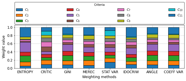
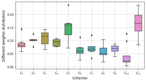
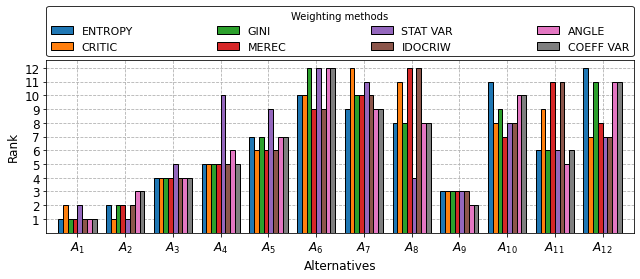
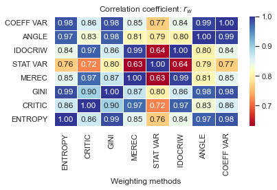
Visualize the results as column graphs of weights, rankings, and correlations.

plot_barplot(df_weights, 'Weighting methods', 'Weight value', 'Criteria')

The PostScript backend does not support transparency; partially transparent artists will be rendered opaque.

plot_boxplot(df_weights.T)

plot_barplot(df_rankings, 'Alternatives', 'Rank', 'Weighting methods')

The PostScript backend does not support transparency; partially transparent artists will be rendered opaque.

results = copy.deepcopy(df_rankings)
method_types = list(results.columns)
dict_new_heatmap_rw = Create_dictionary()

for el in method_types:
    dict_new_heatmap_rw.add(el, [])

# heatmaps for correlations coefficients
for i, j in [(i, j) for i in method_types[::-1] for j in method_types]:
    dict_new_heatmap_rw[j].append(corrs.weighted_spearman(results[i], results[j]))

df_new_heatmap_rw = pd.DataFrame(dict_new_heatmap_rw, index = method_types[::-1])
df_new_heatmap_rw.columns = method_types

# correlation matrix with rw coefficient
draw_heatmap(df_new_heatmap_rw, r'$r_w$')

Stochastic Multicriteria Acceptability Analysis Method (SMAA)

cols_ai = [str(el) for el in range(1, matrix.shape[0] + 1)]

# criteria number
n = matrix.shape[1]
# number of SMAA iterations
iterations = 10000

# create the VIKOR_SMAA method object
vikor_smaa = VIKOR_SMAA()
# generate multiple weight vectors in matrix
weight_vectors = vikor_smaa._generate_weights(n, iterations)

# Calculate the rank acceptability index, central weight vector and final ranking
rank_acceptability_index, central_weight_vector, rank_scores = vikor_smaa(matrix, weight_vectors, types)

acc_in_df = pd.DataFrame(rank_acceptability_index, index = list_alt_names, columns = cols_ai)
acc_in_df.to_csv('results_smaa/ai.csv')

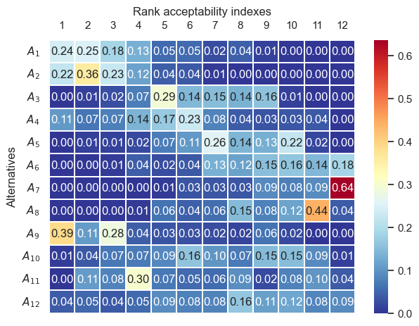
Rank acceptability indexes

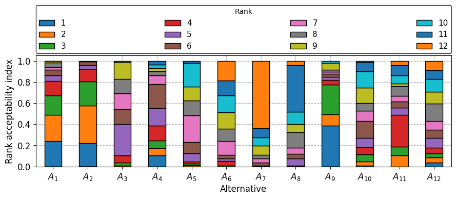
This is dataframe with rank acceptability indexes for each alternative in relation to ranks. Rank acceptability index shows the share of different scores placing an alternative in a given rank.

acc_in_df

	1	2	3	4	5	6	7	8	9	10	11	12
$A_{1}$	0.2395	0.2499	0.1847	0.1341	0.0540	0.0532	0.0240	0.0441	0.0128	0.0037	0.0000	0.0000
$A_{2}$	0.2207	0.3576	0.2252	0.1155	0.0405	0.0351	0.0054	0.0000	0.0000	0.0000	0.0000	0.0000
$A_{3}$	0.0002	0.0102	0.0249	0.0723	0.2924	0.1429	0.1516	0.1359	0.1589	0.0107	0.0000	0.0000
$A_{4}$	0.1063	0.0660	0.0749	0.1386	0.1666	0.2296	0.0797	0.0375	0.0303	0.0348	0.0357	0.0000
$A_{5}$	0.0005	0.0117	0.0142	0.0218	0.0743	0.1069	0.2564	0.1403	0.1311	0.2230	0.0198	0.0000
$A_{6}$	0.0000	0.0009	0.0074	0.0419	0.0242	0.0364	0.1318	0.1158	0.1524	0.1630	0.1418	0.1844
$A_{7}$	0.0000	0.0000	0.0007	0.0013	0.0061	0.0314	0.0344	0.0342	0.0888	0.0766	0.0900	0.6365
$A_{8}$	0.0000	0.0024	0.0025	0.0055	0.0643	0.0438	0.0574	0.1469	0.0771	0.1191	0.4416	0.0394
$A_{9}$	0.3859	0.1073	0.2818	0.0416	0.0312	0.0284	0.0224	0.0168	0.0644	0.0202	0.0000	0.0000
$A_{10}$	0.0095	0.0357	0.0681	0.0707	0.0858	0.1597	0.0998	0.0698	0.1491	0.1512	0.0889	0.0117
$A_{11}$	0.0000	0.1077	0.0799	0.3025	0.0688	0.0538	0.0553	0.0942	0.0214	0.0773	0.1001	0.0390
$A_{12}$	0.0374	0.0506	0.0357	0.0542	0.0918	0.0788	0.0818	0.1645	0.1137	0.1204	0.0821	0.0890

Rank acceptability indexes displayed in the form of stacked bar chart.

matplotlib.rcdefaults()
plot_barplot(acc_in_df, 'Alternative', 'Rank acceptability index', 'Rank')

The PostScript backend does not support transparency; partially transparent artists will be rendered opaque.

Rank acceptability indexes displayed in the form of heatmap

draw_heatmap_smaa(acc_in_df, 'Rank acceptability indexes')

Central weight vector

The central weight vector describes the preferences of a typical decision-maker, supporting this alternative with the assumed preference model. It allows the decision-maker to see what criteria preferences result in the best evaluation of given alternatives. Rows containing only zeroes mean that a given alternative never becomes a leader.

central_weights_df = pd.DataFrame(central_weight_vector, index = list_alt_names, columns = cols)
central_weights_df.to_csv('results_smaa/cw.csv')

central_weights_df

	$C_{1}$	$C_{2}$	$C_{3}$	$C_{4}$	$C_{5}$	$C_{6}$	$C_{7}$	$C_{8}$	$C_{9}$	$C_{10}$	$C_{11}$
$A_{1}$	0.085557	0.068852	0.163567	0.127721	0.120978	0.074311	0.073052	0.079822	0.055629	0.053372	0.097139
$A_{2}$	0.119505	0.091197	0.076790	0.123850	0.056169	0.080498	0.080611	0.079016	0.071870	0.109797	0.110698
$A_{3}$	0.025481	0.024065	0.193722	0.116842	0.152955	0.039404	0.032034	0.020895	0.005310	0.268307	0.120985
$A_{4}$	0.043895	0.085792	0.066643	0.056497	0.065895	0.084770	0.092258	0.084303	0.081521	0.206366	0.132060
$A_{5}$	0.041701	0.283298	0.035020	0.057731	0.051069	0.046757	0.037362	0.032076	0.100242	0.243114	0.071629
$A_{6}$	0.000000	0.000000	0.000000	0.000000	0.000000	0.000000	0.000000	0.000000	0.000000	0.000000	0.000000
$A_{7}$	0.000000	0.000000	0.000000	0.000000	0.000000	0.000000	0.000000	0.000000	0.000000	0.000000	0.000000
$A_{8}$	0.000000	0.000000	0.000000	0.000000	0.000000	0.000000	0.000000	0.000000	0.000000	0.000000	0.000000
$A_{9}$	0.096995	0.115952	0.066120	0.061943	0.105055	0.101578	0.099929	0.104295	0.132537	0.055860	0.059736
$A_{10}$	0.056299	0.030817	0.041581	0.150271	0.045265	0.087209	0.107615	0.080866	0.073499	0.227022	0.099554
$A_{11}$	0.000000	0.000000	0.000000	0.000000	0.000000	0.000000	0.000000	0.000000	0.000000	0.000000	0.000000
$A_{12}$	0.074129	0.038418	0.044376	0.044803	0.044055	0.147604	0.169826	0.132190	0.038341	0.144566	0.121692

Rank scores

rank_scores_df = pd.DataFrame(rank_scores, index = list_alt_names, columns = ['Rank'])
rank_scores_df.to_csv('results_smaa/fr.csv')

rank_scores_df

	Rank
$A_{1}$	3
$A_{2}$	1
$A_{3}$	6
$A_{4}$	4
$A_{5}$	9
$A_{6}$	10
$A_{7}$	12
$A_{8}$	11
$A_{9}$	2
$A_{10}$	7
$A_{11}$	5
$A_{12}$	8

Subjective weighting methods

The illustrative example concerns the multi-criteria problem involving a selection of four alternative sites in Poland for wind farm location regarding ten criteria assessment. The data for this problem used in the procedure for determining the criteria weights in this example and the data on the performance of the alternatives against the evaluation criteria were acquired from the research paper https://doi.org/10.3390/su8080702

# Load data from csv file
data = pd.read_csv('./dataset_localisations.csv', index_col='Symbol')

# decision matrix with alternatives' performance values
df_data = data.iloc[:len(data) - 1, :]

# Criteria types
types = data.iloc[len(data) - 1, :].to_numpy()

# Decision matrix in numpy.ndarray data type required by methods implemented in crispyn package
matrix = df_data.to_numpy()

# Column names
cols = [r'$C_{' + str(j) + '}$' for j in range(1, matrix.shape[1] + 1)]

# Dataframe for weight values determined by different weighting methods
df_weights = pd.DataFrame(index = cols)

df_data

	C1	C2	C3	C4	C5	C6	C7	C8	C9	C10
Symbol
A1	106780	6.75	2	220	6	1	52	455.5	8.9	36.8
A2	86370	7.12	3	400	10	0	20	336.5	7.2	29.8
A3	104850	6.95	60	220	7	1	60	416.0	8.7	36.2
A4	46600	6.04	1	220	3	0	50	277.0	3.9	16.0

AHP weighting method

Construct matrix with criteria pairwise comparison as numpy.ndarray type

PCcriteria_ahp = np.array([
    [1, 2, 2, 2, 6, 2, 1, 1, 1/2, 1/2],
    [1/2, 1, 1, 1, 4, 1, 1, 1, 1/2, 1/2],
    [1/2, 1, 1, 1, 3, 1, 1/2, 1/2, 1/3, 1/3],
    [1/2, 1, 1, 1, 3, 1, 1/2, 1/2, 1/3, 1/3],
    [1/6, 1/4, 1/3, 1/3, 1, 1/3, 1/5, 1/5, 1/9, 1/9],
    [1/2, 1, 1, 1, 3, 1, 1/2, 1/2, 1/3, 1/3],
    [1, 1, 2, 2, 5, 2, 1, 1, 1/2, 1/2],
    [1, 1, 2, 2, 5, 2, 1, 1, 1/2, 1/2],
    [2, 2, 3, 3, 9, 3, 2, 2, 1, 1],
    [2, 2, 3, 3, 9, 3, 2, 2, 1, 1]
])

Calculate AHP weights

# Initialize the `AHP_WEIGHTING` method object
ahp_weighting = mcda_weights.AHP_WEIGHTING()

# Calculate AHP weights passing matrix with criteria pairwise comparison and method of priority vector calculation
weights_ahp = ahp_weighting(X = PCcriteria_ahp, compute_priority_vector_method=ahp_weighting._eigenvector)

# save calculated AHP weights in dataframe for weights
df_weights['AHP'] = weights_ahp

Inconsistency index:  0.006188266444440638

weights_ahp

array([0.11649504, 0.08039711, 0.0614321 , 0.0614321 , 0.02051697,
       0.0614321 , 0.10648668, 0.10648668, 0.1926606 , 0.1926606 ])

SWARA weighting method

Provide vector criteria_indexes (numpy.ndarray type) with indexes of criteria in accordance with given decision problem from \(C_1\) to \(C_n\) ordered in descending order beginning from the most important criterion and vector s including values representing how much criterion (j-1) is more significant than criterion j in percentage in range from 0 to 1

# criteria ordered in descending order from the most significant
criteria_indexes = np.array([8, 9, 0, 6, 7, 1, 2, 3, 5, 4])
# vector s
s = np.array([0, 0.4, 0.17, 0, 0.2, 0.25, 0, 0, 0.67])

# Calculate SWARA weights
weights_swara = mcda_weights.swara_weighting(criteria_indexes, s)

# save calculated AHP weights in dataframe for weights
df_weights['SWARA'] = weights_swara

LBWA weighting method

Construct list with lists (subsets) criteria_indexes of grouped and ordered index of criteria according to their significance beginning from the most important within each subset and list with lists containing influence values of criteria within each subset provided in order beginning from the most significant criteria_values_I. Then calculate LBWA weights using lbwa_weighting function.

criteria_indexes = [
    [8, 9, 0],
    [6, 7, 1],
    [2, 3, 5],
    [],
    [],
    [],
    [],
    [],
    [],
    [4]
]

criteria_values_I = [
    [0, 0, 2],
    [1, 1, 2],
    [1, 1, 1],
    [],
    [],
    [],
    [],
    [],
    [],
    [3]
]

weights_lbwa = mcda_weights.lbwa_weighting(criteria_indexes, criteria_values_I)

df_weights['LBWA'] = weights_lbwa

SAPEVO weighting method

Construct matrix with degrees of pairwise criteria comparison in scale from -3 to 3, then calculate criteria weights using sapevo_weighting function.

PCcriteria_sapevo = np.array([
    [ 0, 1, 1, 1, 2, 1, 0, 0, -1, -1],
    [-1, 0, 0, 0, 1, 0, 0, 0, -1, -1],
    [-1, 0, 0, 0, 1, 0, -1, -1, -1, -1],
    [-1, 0, 0, 0, 1, 0, -1, -1, -1, -1],
    [-2, -1, -1, -1, 0, -1, -2, -2, -3, -3],
    [-1, 0, 0, 0, 1, 0, -1, -1, -1, -1],
    [ 0, 0, 1, 1, 2, 1, 0, 0, -1, -1],
    [ 0, 0, 1, 1, 2, 1, 0, 0, -1, -1],
    [ 1, 1, 1, 1, 3, 1, 1, 1, 0, 0],
    [ 1, 1, 1, 1, 3, 1, 1, 1, 0, 0]
])

weights_sapevo = mcda_weights.sapevo_weighting(PCcriteria_sapevo)

df_weights['SAPEVO'] = weights_sapevo

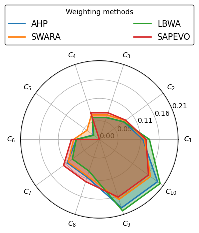
df_weights

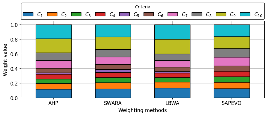
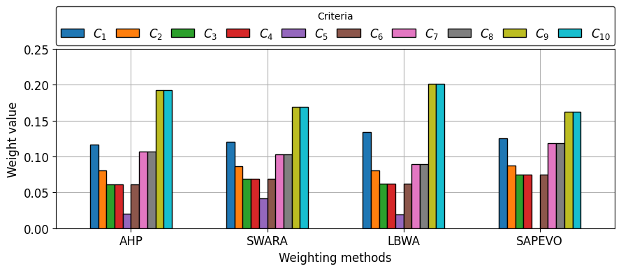
	AHP	SWARA	LBWA	SAPEVO
$C_{1}$	0.116495	0.120886	0.134093	0.12500
$C_{2}$	0.080397	0.086101	0.080456	0.08750
$C_{3}$	0.061432	0.068881	0.061889	0.07500
$C_{4}$	0.061432	0.068881	0.061889	0.07500
$C_{5}$	0.020517	0.041246	0.018711	0.00000
$C_{6}$	0.061432	0.068881	0.061889	0.07500
$C_{7}$	0.106487	0.103321	0.089396	0.11875
$C_{8}$	0.106487	0.103321	0.089396	0.11875
$C_{9}$	0.192661	0.169240	0.201140	0.16250
$C_{10}$	0.192661	0.169240	0.201140	0.16250

Visualize criteria weights calculated with each subjective weighting method in column charts and radar chart.

plot_barplot_stacked(df_weights.T, stacked = True)

plot_barplot_stacked(df_weights.T, stacked = False)

plot_radar_weights(df_weights)

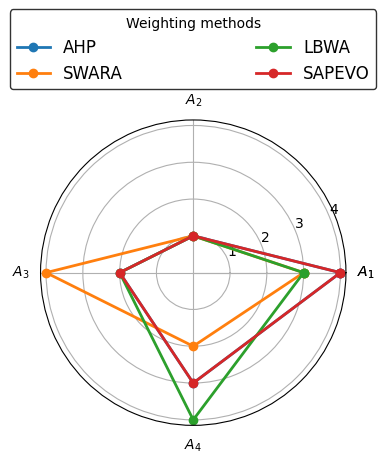
Determine utility function values using the VIKOR method and rank alternatives to generate rankings for each weighting method.

weighting_methods_names = ['AHP', 'SWARA', 'LBWA', 'SAPEVO']
weights_list = [weights_ahp, weights_swara, weights_lbwa, weights_sapevo]

# MCDA assessment
# dataframe for alternatives
alts = [r'$A_{' + str(j) + '}$' for j in range(1, matrix.shape[0] + 1)]
df_prefs = pd.DataFrame(index = alts)
df_ranks = pd.DataFrame(index = alts)

vikor = VIKOR()
for el, weights in enumerate(weights_list):
    pref = vikor(matrix, weights, types)
    rank = rank_preferences(pref, reverse=False)

    df_prefs[weighting_methods_names[el]] = pref
    df_ranks[weighting_methods_names[el]] = rank

df_prefs

	AHP	SWARA	LBWA	SAPEVO
$A_{1}$	0.971262	0.922828	0.863588	0.962927
$A_{2}$	0.000000	0.000000	0.000000	0.000000
$A_{3}$	0.941176	0.941176	0.861822	0.925714
$A_{4}$	0.954106	0.882663	1.000000	0.937836

df_ranks

	AHP	SWARA	LBWA	SAPEVO
$A_{1}$	4	3	3	4
$A_{2}$	1	1	1	1
$A_{3}$	2	4	2	2
$A_{4}$	3	2	4	3

plot_radar(df_ranks)